|
|
| Visite: 1207 | Gradito: |
Leggi anche appunti:The Victorian AgeThe Victorian Age The Victorian Age took its name from Queen Victoria whose SkyscrapersSKYSCRAPERS The skyscrapers are the key to making a modern American cityscape Charles DickensCharles Dickens LIFE Dickens |
 |
 |
Origin of Tomography
The word Tomography has a Greek etymology. Taking its origin from the roots " tomos tomos] which can be translated as "writing" and "grafia" [grapos] which can be translated as "section", this term means to write something that is possible to be observed only from the internal side of a of structure.
The Tomography approach has gained its popularity first as a very important tool for different medical applications. This term has recently given the name to many kinds of medical tests and investigations. For example, the axial computerized tomography, generally known as TAC, is a radiology technique based on a particular system of measurements of the coefficients of absorption of the X-Rays from the fabrics subject to examination in a scanning axial crossroads. This invention changed radically the science of the knowledge of a lot of hidden issues that are incomparably more difficult to investigate than those that could be traced by the direct sight.
But why are these notions being discussed and what is their common aspect with the studies of the Network? The answer to this question can be well illustrated by considering the Internet infrastructure today as the cybernetic equivalent of a human organism. The last miles connection from the Internet to personal computers are similar to thousands of capillaries and small and medium sized Internet service providers (ISPs) are interconnected like the arteries to the backbone transit providers. The global infrastructure of Internet consists, therefore, in a complex array of interconnected telecommunication networks, where each network is a part of an Internetwork, and is very difficult to be diagnostically analyzed. That is why the described analogy can be used here to introduce how the term Tomography can be applied to the Internet world.
The suggested solution is to develop a method for estimating internal behaviour patterns by using the measurements taken at the network edges only, like, for example, exploiting end-to-end traffic to reconstruct the network internal performance. This new types of research were a necessary condition for the continuous growth of the Internet, which was originally a small controlled network in the late 1970's serving the needs of few users and rapidly developed then into a huge multi-layered heterogeneous collection of terminals. This growth required a continuous extension of monitoring techniques able to provide managing it in space and time.
Obtaining the information about network performance, such as link loss rate and queuing delays, plays an important role in isolation of network congestion and detection of performance degradation. The behaviour of the global network, such as routing algorithms, servicing strategies and performance verifications, can benefit from monitoring techniques reporting information. That is why monitoring of large communications system is simply the minimum necessary condition to diagnose all, or at least a part of most important vital components for the efficient network operation.
But why the Tomography can be considered as the exceptional approach the world of the network is looking for? Why cannot the normal internal approach, which has always been used during the Internet growth, continue to be applied?
Internal and External Measurements
It is important to differentiate between the common internal approach and the external trade motif of Tomography science. Internal direct measurements are made within the network elements, as, for example, packet lost, delay or traffic characteristics, inside the network. External measurements are made along the network on the end-to-end or edge-to-edge paths. From Figure 1 it is possible to realize the basic difference of measurements between these two approaches.
Internal approach is becoming irrelevant because of the high number of its potential limitations. The measurement process imposes potential load to the network. In fact, the cooperation between internal servers or routers can lead to impracticable overhead in terms of extra communication requirements and coordination efforts. Besides, the measurements access can be limited by service providers, because, for example, they might consider such kind of information as highly confidential, therefore, some administrative problems can take place. Finally, internal measurements investigate the average behaviour, especially the throughput or average queuing with a restricted number of possible statistics.
For these reasons, external approach has the most important advantage: it allows to carry out the measurements that do not require a dedicated cooperation from internal network devices and minimize the network load. These aspects can be overcome by means of tomography.
Studying and monitoring the network by means of making the measurements only at the network edges lead to the lack of cooperation between the internal devices, which, in turn, can be the reason for the waste of resources. Computing and elaborate these measurements from two dedicated external calculators on the edge provide with the opportunity of separation between network and its management.
Figure 1: Internal measurement, is made directly between two elements of the
network. External, is obtained indirectly from the measurement along a path,
from host 1 to host
Topics of Network Tomography Approaches
With the emerging of Internet tomography there appeared a broad new science of reporting several groups of methods to investigate inference of internal network behaviour based on external end-to-end network measurements. This approach is based on the inference theory, the goal of which is to obtain "less price" network statistics revealing hidden network structure and helping to detect isolated congestion, routing faults or anomalous traffic.
The term tomography can have different meaning depending on the branch of studies it is being applied for. It can be used as a tool for the following areas:
Link-level delay estimate
Inference of the probability distribution on links along global path, where the measurements are made. An experimental application in a LAN (Local Area Network) is mentioned in this text (Section 5).
Link load at limit and Throughput
Estimates link load limit, allows to manage possible congestions or bottlenecks, knowing the traffic intensity estimate.
Topology identification (Topography)
Estimate of the internal network connectivity and estimate of the topology configuration. These are some of the most important applications showing how the "inference" world can use its complex tools, for the estimation of a large number of spatially distributed parameters[1].
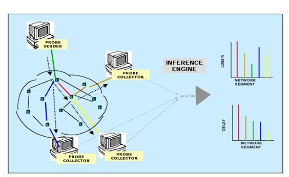
Figure 2: The collection of the measurements along the network are input for large-scale inference strategies to estimate some parameters of the network, like the probability loss rate or delay distribution of internal links[2].
The most difficult task is to adopt the simplest possible model to a large-scale estimation, taking into consideration the error under the minimum upper bound request. It is essential to know the degree of the reliability of an estimation.
Often the accuracy can be considered as the equivalent to increase in computation efforts, requiring the application of an intricate analysis of network, which is a complex and difficult to estimate algorithm process. Usually, it is better to use a more simple model, because the results of it will be sufficient for inference of the performance characteristics. It is important to have a trade-off between the accuracy and computations to be able to apply these results to the network.
Tomography approach enables to move the focus from a detailed real analysis of the network (as, for example, queuing or traffic modeling) to a set of measurements and large scale inference strategies. This aspect is shown in the Figure
The measurements play here a very important role. Tomography approach must be able to avoid conditioning the same network by the measurements, which may be Passive or Active. The passive measurements use the existing traffic along a path in the network. To conduct the measurement it is necessary to sample the network traffic flow. The active measurements are used to generate a traffic flow and notify the network behavior. These are two different kinds of measurement, and the use of them depends on the ability to apply it to the network. Both approaches play an important role because they do not overload the system being used to obtain measurement with a sufficient reliability. For example, in case of passive measurement, the sample is not influenced by a particular state of the network. It is important to conduct measurement independently from the spatial and temporal structure. Probe tools, on the contrary, are necessary to apply for active measurement.
The first important conclusion can be made: network tomography is a science able to capture a network performance adjusting the active or passive measurement to an inference strategy.
4 Basic Definitions
Getting to the core of a network it is possible to recognize several different structures along a large scale network. They are the basic definitions, but are fundamental to explain and define in the inference method. The simplest way to depict a network is shown in Figure 3. The goal is to visualize the connectivity topology of a large and widely spread network. Each node can represent a computer terminal, router or subnetwork, depending on the accuracy level of the logical representation. The connection between two adjacent nodes is called link. A link is a direct connection between two nodes. The union of adjacent links defines a path. This is a logical representation, where each logical link is a chain of physical links connected by routers. Each path is built by a source-node and a destination-node. To identify the measurement on this path, the source-node transmits a message (packets) to the destination-node, passing through several nodes sharing the same path. A possible inference strategy is to use the obtained measurement and to carry out some internal link characteristics, such as loss rate estimation or link delay estimation. If a path is defined, there exist two forms of tomography approach, depending on the hierarchical structure level of the network.
i. Link-level parameter estimation
In this context, the target of tomography strategy is the estimation of parameters belonging to links, such as time delay estimation. The goal is to estimate the time delay necessary to cross a link along a path, having the measurement on the integer path. It is an extremely challenging task if the possible reasons, which make the real time swing, are taken into consideration. The time delay can have many random components determining the behavior, ranging from the propagation delay, to the queuing at the router and router packet servicing delay, bearing in mind the possibility of the packet dropped event. This happens, usually, due to the overload of finite output buffer of the routers across the link or power failures.
ii. Path-level traffic intensity estimation
It is an estimate operating on a higher hierarchical level. Usually, this approach focuses on the traffic intensity estimation crossing all paths in the network. The measurements consist of counts of packets that pass through the nodes, combining all the possible origin-destination paths. This represents a global approach to measure the network. The complexity increases not only for the random measurement along each path, but also due to the fact that there exist no fixed paths in the network.
Figure 3: The collection of the measurements along the network are input for large-scale inference strategies to estimate some parameters of the network, like the probability loss rate or delay distribution of internal link [2].
The first model is of lower complexity. It can be applied, for example, to conduct the estimations in a LAN. This approach is used in the practical application enounced in Chapter 6.
A large scale network can be represented by many mathematical models, the goal of which is to simulate its real behavior. It is possible to resolve many Network Tomography problems with the help of these models. In this work there will be given a short description of Linear Model.
5 Linear Model
Linear model is a rough approximation of a Network Tomography inference problem
Y = A q e (1)
where y is a vector of the measurement, and each component can represent, for example, end-to-end delay, or packet counts, depending by the inference strategy adopted. A represents the Routing Matrix or Traffic Matrix. q is a vector of quantities which lead information, which are usually the parameters to estimate, such as mean delay, logarithms of loss rate, or packet transmission probability over a link. e is an addictive vector error which absorbs all the error effects, from measurement errors in vector y or from the parameter estimation q
A is a
binary matrix, which capture the topology of the network. Figure 4 depicts a
simple example showing how this matrix is constructed. The i, j-th element is
equal to 1 only if there is the connection between nodes i and j. Using the
topology it is possible to consider the example of
unicast loss rate tomography. The goal is to
obtain the measurement of the probability of a packet right transmission over a
link, which can be seen in the Figure 5, using active measurement. Packets are
sent by the sender 0 and received by the nodes 2 and 3. ![]() and
and ![]() denote the number of packets sent and received by receiver node k.
Measurements are obtained simply by the number of the packets arrivals and
define the packet arrival probability
denote the number of packets sent and received by receiver node k.
Measurements are obtained simply by the number of the packets arrivals and
define the packet arrival probability ![]()
![]() for j =1,2,3 represents the parameter associated with each link to be estimated.
This is a simplified example and the error e is ignored.
for j =1,2,3 represents the parameter associated with each link to be estimated.
This is a simplified example and the error e is ignored.
Figure 4: The matrix A is generated allowing 1 where exists a link along the
i-th path.
The particular application is shown in the equation
 (2)
(2)
Large scale network inference estimates the network parameter q if y is being measured. Although it is a simplified inference model, it represents a lot of complex aspects. Usually q vector is replaced by an x vector function of q, parameter to estimate. x represents a measurable quantity containing the hidden parameter to estimate. Each component of x vector depends from the respective q component.
![]()
![]() j= 1,..,J (3)
j= 1,..,J (3)
This relationship may be more or less complex and depends on the inference strategy. Besides, as it can be noticed from the Equation 2, this dependence is a rough approximation, which add, an error to the estimated results. This correlation must be only clear enough.
Figure 5: y represents the measurements at the end hosts. ![]() represents
the parameter to estimate over j-th link.
represents
the parameter to estimate over j-th link.
Another important point of the linear model is the time dependence. In fact, all the variables of the Equation 1 are time-dependent. This scenario reflects the dynamical nature of the real network, which increases the complexity of the described model.
yt = A xt + et
The matrix A depends on time, too, but can also be assumed independent in the first approximation under the hypothesis of knowledge of the topology of the network. That is why the estimation problem involves tracking time-dependent parameters. yt becomes a vector of measurements recorded at given time t at a number of different measurement sites.
The target of the inference strategy is to estimate x, and then the respective dependent parameter q. This is a specific case of inverse problem. But the real dimension of A can range depending on different sizes of the network. In a small network, such as shown in Figure 4 , A is a 2 x 3 dimension matrix, with two packet parameters and two measurements sites. But A can reach up to ten thousands of rows and columns for a large subnet of the Internet. The methods to solve this inverse problem depend not only on the matrix A, but also on the nature of the error e. Its components are assumed to be independent, with Gaussian, Poisson, binomial or multinomial distribution. The nature of this error can change the inference strategy, either reducing or increasing the inverse problem. Gaussian distributed noise with covariance that is independent of Aq allows to use the recursive linear least squares methods and other iterative equations solvers. This is the most simple case for computation, but is also the most rare one. In fact, usually the error is Poisson, binomial and multinomial distributed and more sophisticated statistical approach is required, as, for example, the use of non-linear least squares methods, maximum likelihood approach with expectation-maximization algorithm (EM) or maximum at posteriori algorithm (MAP)[3]. This recursive algorithm requires the inverse of matrix A, but usually A is not of full rank (for example, in Equation 2) which increases the mathematical computation. This scenario shows the degree of complexity of the inference field and the necessity to choose the right strategy for parameter estimation. In fact, the most important is to reach the trade-off between statistical accuracy and computational overhead. The statistical accuracy is required to obtain an estimate error within the prefixed bound, without too complicated computational efforts.
Another approach of inference strategy is the Maximum Likelihood Estimation (MLE). MLE gives good results in terms of efficiency but is too difficult to calculate [3,4]. That is why it has been recently replaced with the maximum pseudo likelihood estimation (MPLE)[1,5]. This approach reduces the computational burden and provides the good statistical efficiency.
The basics of the inference model will be described in next paragraph and this approaches will be described.
6 Inference Model
The goal of the inference model is to attribute a value to an unknown parameter using a statistics of measurement. The estimates are necessary when the parameter cannot directly be measured. Usually, the parameter is, as in the example described above, a multidimensional vector of parameter. Therefore, the goal will be to estimate the vector of these parameters. It is preferable first to study a general one-dimension parameter estimate and then to extend these notions to the multidimensional case.
Let q the real parameter to estimate and
Y the measurement, the estimate of which is being constructed. Y is a vector of N samples (at
different time) ![]() or a continuous observation within a given time interval. The target is to
give a value to the parameter using N samples
or a continuous observation within a given time interval. The target is to
give a value to the parameter using N samples ![]() of the integer observation. Each
component
of the integer observation. Each
component![]() , the
sample of the measurement, represents identical random variable. It is possible
to define the probability density function f (y; q), which expresses the dependence of
data y from the parameter q
, the
sample of the measurement, represents identical random variable. It is possible
to define the probability density function f (y; q), which expresses the dependence of
data y from the parameter q
Figure 6 depicts a general estimate process. A source
of parameters generates a vector q, identifying a point in the parameters space.
This means that the target of the inference estimate has been fixed. The data
measurements Y are points of the
observations space. Each measurement generates a specific point in this space.
The function f(y; q) expresses the statistic connection between
these spaces. Using these data the inference strategy should be focused to
discover the value of the parameters adopting an estimate rule ![]() =g(y). Function f(y; q) plays a very important role in
this application. This function represents the probability density of data if
the parameter to estimate varies. It is actually a group of density probability
functions, because each of them corresponds to a different value of the
parameter. The knowledge of this
function allows to apply the method of statistic inference called Maximum Likelihood
Estimation method (MLE).
=g(y). Function f(y; q) plays a very important role in
this application. This function represents the probability density of data if
the parameter to estimate varies. It is actually a group of density probability
functions, because each of them corresponds to a different value of the
parameter. The knowledge of this
function allows to apply the method of statistic inference called Maximum Likelihood
Estimation method (MLE).
Figure 6: General estimate process. A parameter source generates a vector of parameters to estimate, defined in a parameter space. The measurements define the linking function f(Y;q) between two space to obtain the estimator of the vector of parameters [3].
Given a sample of measurement a point in the observation space is defined (Figure 6). After this observation the estimate can be obtained by choosing the value of the parameter which has given the measurement y with the highest probability.
The Maximum Likelihood Estimate (MLE) is the estimated value ![]() , at
which the sample of measurement
, at
which the sample of measurement ![]() gives the maximum probability
density function f(Y=y; q
gives the maximum probability
density function f(Y=y; q
When Y is observed, f(Y=y; q)=L(q) becomes the function of the only
parameter q to
estimate. It represents the maximum
likelihood function which is to be maximized to obtain the value ![]() .
Under the independence hypothesis of the random variables
.
Under the independence hypothesis of the random variables![]() , the
maximum likelihood function is
, the
maximum likelihood function is
![]() (5)
(5)
and the maximum likelihood estimate is the parameter which maximizes this function
![]() (6)
(6)
where arg represents the argument of the function L(q
The Figure 7 depicts the case of a mean estimate of a random variable with normal distribution. For the given measurement there should be defined the interval where the parameter which gives the maximum of L(q) has to be chosen.
Figure 7. If the measurements are
contained in (x, x+Dx), the
estimate more likelihood of the parameter q is ![]()
The maximum likelihood estimate gives statistically good results and it is characterized by the following basic properties: Unbiased [3], Efficient[3], Consistent[3].
Unbiased ![]() . An
estimator is unbiased if the average on the number experiments of
. An
estimator is unbiased if the average on the number experiments of ![]() gives a result equal to the true value of q
gives a result equal to the true value of q
Efficient: An estimator is efficient if it is unbiased and its variance reaches the Cramer-Rao Bound (CRB).
Consistent ![]() and
and ![]() . An
estimator is consistent if it improves the performance of its estimation when
the number of samples increases.
. An
estimator is consistent if it improves the performance of its estimation when
the number of samples increases.
In the multidimensional approach the
parameter is replaced by a vector of
parameter ![]() .
The measurements are the components of the vector
.
The measurements are the components of the vector ![]() This approach is basically the same, although
the mathematical efforts increase. Maximum likelihood estimate represents the
unknown location of the point in the multidimensional parameter space, given
the vector of vectors Y of the
measurements. In this context maximum likelihood function is a multidimensional
one, depending on the vector of parameters q
This approach is basically the same, although
the mathematical efforts increase. Maximum likelihood estimate represents the
unknown location of the point in the multidimensional parameter space, given
the vector of vectors Y of the
measurements. In this context maximum likelihood function is a multidimensional
one, depending on the vector of parameters q ![]() represents the set of parameters which have
given the measurement
represents the set of parameters which have
given the measurement ![]() with the higher probability. In the described
application vector
with the higher probability. In the described
application vector ![]() can represent the result of an inference
strategy in a link-level delay estimation. Each component j is the delay estimate on j-th
link.
can represent the result of an inference
strategy in a link-level delay estimation. Each component j is the delay estimate on j-th
link.
Now it is important to link maximum likelihood approach to the practical application and to introduce a variant called Maximum Pseudo Likelihood Estimate (MPLE). This approach has the same statistical characteristics as the maximum likelihood, but is much easier to compute, especially by adopting a linear model.
7 Maximum-Pseudo Likelihood Approaches
Consider the linear model of the Equation 1 omitting the error e
Y= A X
![]() is a J-dimensional vector. Each
component represents the dependence of the parameter to estimate through the
density function
is a J-dimensional vector. Each
component represents the dependence of the parameter to estimate through the
density function ![]()
![]()
![]()
![]() j=1,..,J (8)
j=1,..,J (8)
The goal is to estimate networks
dynamic parameters, such as link delay or traffic flow counts, obtaining X and
then, if![]()
![]() is
known, to estimate the j-th parameter. In this application the independence of
all the components of X is required.
This is the necessary assumption for the application of likelihood approaches.
is
known, to estimate the j-th parameter. In this application the independence of
all the components of X is required.
This is the necessary assumption for the application of likelihood approaches.
![]() is a
I-dimensional vector of measurements. A is
the routing matrix, as shown in Figure 4. The example of this application is
demonstrated in Figure 8. This is an arbitrary multicast tree with four
receivers. It is multicast, because in this application root sends a packet
probing to all the receivers[6]. In this case it can be noticed in Figure 9 how
the Equation 7 can be applied. Each component Yj represents the one way delay
measured from the root to node j. The connection between node i and its parent
defines link i. Matrix A is
given, because the topology of the network is known. It is obtained with a spanning tree
algorithm. It is a I x J matrix, so there are I receivers and J internal links.
Therefore, Y1,..,Y4 are the measurements (at nodes 4-7), and X1,..X7 are the
delays over internal links 1-7.
is a
I-dimensional vector of measurements. A is
the routing matrix, as shown in Figure 4. The example of this application is
demonstrated in Figure 8. This is an arbitrary multicast tree with four
receivers. It is multicast, because in this application root sends a packet
probing to all the receivers[6]. In this case it can be noticed in Figure 9 how
the Equation 7 can be applied. Each component Yj represents the one way delay
measured from the root to node j. The connection between node i and its parent
defines link i. Matrix A is
given, because the topology of the network is known. It is obtained with a spanning tree
algorithm. It is a I x J matrix, so there are I receivers and J internal links.
Therefore, Y1,..,Y4 are the measurements (at nodes 4-7), and X1,..X7 are the
delays over internal links 1-7.
Figure 8: A multicast tree, with four receivers. A root sends a packet to all four receivers.
Figure 9: A path is defined from the
root to the end host . It is possible to obtain four paths. Each link
measurements is represented by ![]()
![]()
The goal of the maximum likelihood strategy is to estimate the components of q, given the measurement Y and using the dependence of the Equation 7 and the Equation 8. From the probability density f(Y; q) for this application in Figure 8 the maximum likelihood function is obtained when the measurement has been fixed.
![]() (9)
(9)
The main problem is that a
multidimensional maximization requires a lot of efforts when the number of
variables to estimate increases. This example is a simplified case with seven
unknown values. If this strategy will be applied to a bigger network, the
maximization algorithm will become more complex. Estimating the vector ![]() means, in fact, resolving a multidimensional maximization
problem, the essence of which is to find a multidimensional vector with
components that represent a point of maximum. Usually this research is
conducted using the iterative algorithm, such as Expectation Maximum algorithm
[7,8]. After a number of steps the algorithm reaches a stationary point, which
does not change from one step to another. It represents the result of the
maximization. The problem is contained in the number of steps required from the
algorithm. If the dimension of the vector to estimate increases, the number of
steps increases, too. Besides, there is an inevitable loss of accuracy and it
is more relevant when the dimension of the vector increases. If the estimate is
required for a real time service, this application cannot be used. The
requested time is too long and depends on the dimension of the network. To be
less restricted by these boundaries a variant of the maximum likelihood
function, which is called pseudo maximum likelihood function, should be
introduced.
means, in fact, resolving a multidimensional maximization
problem, the essence of which is to find a multidimensional vector with
components that represent a point of maximum. Usually this research is
conducted using the iterative algorithm, such as Expectation Maximum algorithm
[7,8]. After a number of steps the algorithm reaches a stationary point, which
does not change from one step to another. It represents the result of the
maximization. The problem is contained in the number of steps required from the
algorithm. If the dimension of the vector to estimate increases, the number of
steps increases, too. Besides, there is an inevitable loss of accuracy and it
is more relevant when the dimension of the vector increases. If the estimate is
required for a real time service, this application cannot be used. The
requested time is too long and depends on the dimension of the network. To be
less restricted by these boundaries a variant of the maximum likelihood
function, which is called pseudo maximum likelihood function, should be
introduced.
The main idea of this method is to decompose the original model into a series of simpler subproblems and to construct the pseudo-likelihood function by multiplying the marginal likelihoods of such subproblems. One of them is obtained by selecting the pairs of rows from the routing matrix A. Let S be the set of subproblems obtained by selecting all the possible pairs of rows from the I x J matrix A.
A: S = (10)
For each subproblem sIS the observed subvector is obtained.
![]() (11)
(11)
 (12)
(12)
![]() is
the vector which contains the variables to estimate for the subproblem s using the Equation 11.
is
the vector which contains the variables to estimate for the subproblem s using the Equation 11. ![]() represents
the subrouting matrix selecting rows
represents
the subrouting matrix selecting rows ![]() and
and ![]() . For
each s let
. For
each s let ![]() the marginal likelihood function with
the marginal likelihood function with ![]() the
parameters of s. The hypothesis of independence
of subproblems defines the pseudo-likelihood function as the product of the
marginal likelihood functions of all the subproblems. The Equation 13 shows the
pseudo-likelihood function.
the
parameters of s. The hypothesis of independence
of subproblems defines the pseudo-likelihood function as the product of the
marginal likelihood functions of all the subproblems. The Equation 13 shows the
pseudo-likelihood function.
![]() (13)
(13)
Let ![]() the log-likelihood function of subproblem s, the pseudo log-likelihood function is
defined as
the log-likelihood function of subproblem s, the pseudo log-likelihood function is
defined as
![]() (14)
(14)
Maximum of this
function represents the Maximum Pseudo-Likelihood Estimation (MPLE) of
parameters ![]() . The
Pseudo function allows to divide the analyses of the global parameter
. The
Pseudo function allows to divide the analyses of the global parameter ![]() in some marginal analyses, which is the great
advantage of this method. In fact, it allows to conduct a number of simpler
computation, as, for example, to investigate several subproblems, instead of
conducting a complex investigation. Using pseudo-EM algorithm, which is a
variant of EM-algorithm, it is possible to maximize pseudo likelihood
function[9].
in some marginal analyses, which is the great
advantage of this method. In fact, it allows to conduct a number of simpler
computation, as, for example, to investigate several subproblems, instead of
conducting a complex investigation. Using pseudo-EM algorithm, which is a
variant of EM-algorithm, it is possible to maximize pseudo likelihood
function[9].
Let ![]() be the log-likelihood function of the
subproblem s if all the data are
given. It is the likelihood function of the dependence in the Equation 8.
be the log-likelihood function of the
subproblem s if all the data are
given. It is the likelihood function of the dependence in the Equation 8.
Let ![]() be
the estimate of q
obtained in the k-th step. The iterative function
be
the estimate of q
obtained in the k-th step. The iterative function ![]() is maximized in k+1 steps, until it reaches a stationary value of
is maximized in k+1 steps, until it reaches a stationary value of ![]() . It
is defined as
. It
is defined as
![]() (15)
(15)
The investigation of this maximum multiplies many subexpectations. A subexpectation represents the expectation of a subproblem. This is the main advantage of MPLE. The right choice of the starting point for this iterative algorithm makes it easy to reach faster the estimate.
Figure 10 shows how a marginal likelihood function is obtained. A subproblem consists in the choice of a subtree considering only two receivers. If I is the number of end receivers, there are I(I-1)/2 subtrees. Configuration of a subtree is equivalent to selecting two rows of the matrix A. Figure 11 can be used as an example for a larger network. The the hypothesis of independence, it is necessary to come back to the global model only to
Figure 10: A subproblem is identified selecting two rows of the matrix A. This choice is equivalent to identify two end receivers.
![]()
![]()
multiply all the subtrees. This assumption is required, even if it does not represent the reality, where usually the subproblems are dependent.
Figure 11: When two end receivers are chosen a subtree is identified, and it is more simple to calculate the marginal likelihood function for this subproblem.
8 Computational Complexity
Usually maximum likelihood method is
infeasible for real size networks. It observes all possible internal delay
vectors X. The conducted studies
show that the computational complexity grows at a non-polynomial rate [1]. The
Pseudo likelihood method, on the contrary, reduces this augment. To compare
both methods it is necessary to apply them to a small network as shown in the
Figure 8. In this case the performances of MLE and MPLE are comparable. MPLE is
more robust than MLE, because it has a smaller standard deviation of the error
generated in each estimate. This is a consequence of the partition adopted in
the pseudo method. The Pseudo function, in fact, is a product of less complex
likelihood function on subproblems. N is
the number of edge nodes, where the measurements are made, and complexity is the
number of operations to be computed. The complexity of MLE is proportional to ![]() and, in case of MPLE, to
and, in case of MPLE, to ![]() [1].
For this reason a small network can be compared by complexity, but not a larger
one.
[1].
For this reason a small network can be compared by complexity, but not a larger
one.
Another performance to test is the computational speed. MPLE is faster than MLE, because a matrix of a subproblem has a smaller dimension than the total matrix. This difference in time increases when the number of edge nodes increases. Pseudo likelihood is a variant of the normal likelihood model, and it becomes really important when the size of the network increases. In a LAN (Local Area Network) the models are equivalent. In this work there is described the likelihood model with a maximum expectation algorithm to obtain a link-delay estimation on a LAN. To introduce the both of them it is necessary to have a global vision of this scenario. It can be a valid variant whenever the dimension of the network to analyze is huge.
Besides, the goal is to use a model without any a priori information, which could be helpful for the estimation. This is the case of the MAP model (Maximum a Posteriori)[3]. Measurement from the edges will be then the only available information.
|
| Appunti su: |
|
| Appunti Tedesco |  |
| Tesine Spagnolo |  |
| Lezioni Francese |  |